Placeholder Image

Subtitles section Play video

  • MALE SPEAKER: Good afternoon.

  • Thanks, everybody, for coming from the remote sites

  • to attend the talk by John Martinis about the design

  • of a superconducting quantum computer.

  • And we're very pleased to have John

  • here with us, just a short ride from UC Santa Barbara.

  • And the reason we are excited is John

  • is considered one of the world, if not THE world

  • authority, on superconducting qubits.

  • So since the current machine we're working on

  • is based on superconducting qubits, of course,

  • his opinion and advice would be very important

  • for the guidance of our project.

  • So John got his PhD in physics in 1987

  • from UC Berkeley in California.

  • But then went to France to the Commisiariat Energie

  • Atomic in Saclay.

  • Afterwards, he worked in NIST in Boulder.

  • And then in 2004, he settled where he is right now,

  • being full professor at UC Santa Barbara.

  • And then in 2010, nice achievement,

  • getting the AAAS Science Breakthrough of the Year

  • award for his work on a quantum mechanic oscillator.

  • So we are very curious to hear your--

  • JOHN MARTINIS: OK.

  • Thank you very much.

  • MALE SPEAKER: Oh, one last thing I should say

  • is you remote sites, when the talks over, at this time

  • you guys will be able to ummute, and then you

  • can ask questions remotely.

  • Thank you.

  • JOHN MARTINIS: Thank you very much for the kind invitation

  • to come here.

  • I have a son who's a computer science major at UC Berkeley.

  • And I don't know if you have kids.

  • When you have kids and they're young,

  • the parents can do no wrong.

  • And then they turn into teenagers,

  • and their esteem of you goes down.

  • And then, as they get into the real world,

  • you suddenly become more and more intelligent

  • for some reason.

  • So coming to Google, for my son, is totally cool.

  • Makes me totally cool.

  • So I'm at a much higher esteem today after doing this.

  • I want to talk about our project now

  • to work on superconducting qubits.

  • And to talk about some recent, kind of amazing results here.

  • This is maybe one of the first times

  • we're talking about these results.

  • The ideas of quantum computing have been around

  • for 20, 25 years or so.

  • The idea here is you can do some kind of calculations

  • maybe much, much more powerfully than you can ever

  • do with a classical computer, taking

  • advantage of quantum states.

  • But it's been 20 years or so.

  • And you might ask, well, is it really

  • possible to actually build a quantum computer?

  • It's maybe a theorist's dream.

  • Or I've heard one paper call it a physics nightmare

  • to build a quantum computer.

  • It's really hard.

  • We've been going at it for 20 years.

  • Are we really going to get there?

  • Is it possible?

  • And what I want to do is talk today

  • about some theoretical understandings

  • in the last few years, and some recent results

  • in the last year.

  • Really coming up to data-- I'm going

  • to show data we've taken in the last few weeks.

  • Where we really think we can build a fault-tolerant quantum

  • computer.

  • And we can start down a road to really harvest,

  • to take advantage of the power of quantum computation.

  • So I'm going to talk about the theory.

  • I'm going to talk about our new superconducting qubits.

  • Basically, here, with the theory for fault-tolerant quantum

  • computer, you have to make your qubits well,

  • with an error per step of about 1%.

  • Then you can start building a quantum computer.

  • I'm going to show here that, in fact, we've done that.

  • To motivate this, I want to talk a little bit about D-Wave,

  • because people at Google and elsewhere

  • are thinking about that.

  • And exponential computing power.

  • And then a little bit more about the need

  • for fault-tolerant computer computation to do this.

  • So let's just start with the D-Wave Here's their machine.

  • Beautiful blue picture here.

  • They've been very clever in their market

  • to solve optimization problems, essentially

  • mapping it to physics of what's called a spin glass.

  • And one of the big conjectures of the D-Wave machine

  • is, because they're doing this energy minimization

  • optimization, mapping it to this physics problem,

  • maybe you don't have to build a quantum

  • computer with much coherence at all.

  • And in fact, their machine has about 10,000 times less

  • coherence then the kind of devices we're talking here.

  • So it's a different way of looking at it.

  • And the nice thing is, once you make that conjecture

  • and assumption, it's not too hard to go ahead and use

  • standard Josephson junction fabrication

  • and build a device to try to do that.

  • So it's an interesting conjecture.

  • The machine has superb engineering.

  • It really is a very, very nice piece of work,

  • with the low-temperature physics involved in all that.

  • The problem is, well, although they

  • think they could be useful, a lot of physicists

  • are very skeptical of whether it will have exponential computing

  • power.

  • And I've been enjoying talking to people here at Google

  • and other places, because they've said, well,

  • what does nature have to say in this?

  • So they've actually taken the machine

  • and done some experiments.

  • And I'm just going to review the experiments here.

  • And this is basically the system size versus the time

  • that it takes for the D-Wave machine

  • to anneal to, effectively, the ground state.

  • You're doing the spin glass problem

  • with random couplings between the spins.

  • And they're plotting a typical mean execution time.

  • And with the D-Wave machine, initially

  • for small numbers up to maybe 100, it was pretty flat.

  • But now the latest results, up to 512.

  • It's starting to grow exponentially.

  • This exponential growth is actually

  • matched by some quantum-simulated annealing--

  • both to stimulated, classical annealing and other methods.

  • So the preliminary results here, maybe for this particular class

  • of problems, it's no faster than classical code.

  • Although people are looking at it.

  • That's not a firm conclusion yet.

  • And one has to do more work to see exactly what's going on

  • in the D-Wave and can you use it.

  • We're going to take an approach that's

  • very, very different than this D-Wave machine.

  • It's the conventional, classical approach where physicists

  • have proved theoretically-- it's still only theory--

  • but they have a very strong belief

  • they should be able to build a computer

  • with exponential power.

  • Let me just explain that briefly.

  • It's easy to understand.

  • You take a regular computer, and the classical computer

  • scales linearly with, say, the speed of the processor

  • or the number of processors.

  • It's very well understood.

  • The beauty of CMOS is that the growth of this power

  • actually goes exponentially in time because of the technology

  • improvements.

  • But it's linearly with, say, speed or processor number.

  • However, in the quantum computer,

  • this power grows exponentially.

  • And the basic way to see this is, in a quantum computer,

  • it's not just a 0 or a 1 state.

  • You can put it in a superposition of a 0 and 1

  • state.

  • Just like you say that the electron is orbiting

  • around an atom, and it can be on one side

  • of the atom or the other.

  • There's an electron cloud.

  • At the same time, you can have these quantum bit states

  • that are both 0 and 1 at the same time.

  • So here, for example, we take three quantum bits, put it

  • as a superposition, a 0 and 1.

  • You write that out.

  • You have 8 possible states that the initial state can be in.

  • And you're in a quantum linear superposition

  • of all those states.

  • And the idea is you take this one state,

  • you run it through your quantum computer,

  • and that's basically taking all the 8 possible input states

  • and parallel processing them in one operation

  • through the computer.

  • So the quantum computer allows you

  • to do amazing parallel processing here

  • as 2 to the 3, 8 states, or in general 2 to the n states.

  • So if you have some quantum computer with 64 bits,

  • you're processing 2 to the 64 states at once.

  • To get a doubling in power, what do you do?

  • Here you would you double the size of it.

  • Here, to double the power with a quantum computer,

  • you just add 1 more bit.

  • And you've just double the parallel processing power.

  • And by the time you get something

  • like the 200 quantum bit quantum computer, the parallelization

  • that you're doing is greater than 2 to the 200,

  • is greater than the number of atoms in the universe.

  • So you're clearly doing something there that's amazing.

  • The problem, however, is that you're

  • doing this parallel processing.

  • But you only get, when you measure

  • the system, end bits of information.

  • And you have to encode the problem

  • and only can solve certain problems

  • to take advantage of that kind of optimization.

  • So I'm not going to go into that very much here.

  • But I am going to talk about one application of this.

  • It turns out the government's interested in this.

  • And that is factoring a large number

  • into its component primes.

  • For example, take the idea of factoring a 2000-bit number.

  • The algorithms for doing that scales exponentially.

  • And right now, if you take a 640-bit number,

  • that takes about 30 CPU years to factor that

  • into the composite primes.

  • And then, if you say, OK.

  • You take this and you exponentially

  • scale up to some number like 2000-bit,

  • which is something you might think of doing,

  • what do you have to do to get there?

  • So what I've drawn here is I think

  • this is some Google supercomputer here.

  • I put this especially for this talk.

  • What would you have to build to factor a 2000-bit number?

  • You would have to basically build

  • a computer farm almost the size of North America.

  • And you see, I put it up in Canada.

  • You get natural cooling.

  • Not too many people there.

  • I think the polar bears would be happy for that to be there,

  • because there'd be a lot of people to eat

  • and that'd be good for them.

  • But with that size, if you built something that size,

  • you could do this problem in a 10-year run time.

  • It's possible with that size.

  • However, that's maybe 10 to the 6 trillion dollars.

  • Which, even with quantitative easing,

  • I don't know if the federal government could even do that.

  • It takes about 10 to the 5 times the world's power consumption,

  • and it would consume all of the Earth's energy in one day.

  • So I know Google, you like to think big.

  • But I'm going to just conjecture you're not

  • going to want to do this.

  • This is not practical.

  • I get this example because I want to show you just

  • how reasonable a quantum computer might look.

  • And we don't quite know how to build that now.

  • We have a general idea.

  • We need about 200 million physical qubits.

  • 100,000 let's call logical qubits.

  • You could probably put this in some building size.

  • Maybe even fit in this particular lecture room,

  • with a bunch of refrigerators and control electronics.

  • Maybe a small supercomputer.

  • A 24-hour run time.

  • I don't know what these facts are,

  • but it'd probably be the cost of a satellite or two

  • and certainly not consume that much power.

  • So it's something you could imagine possibly

  • doing, if you understood all the technology on how

  • to build this.

  • The basis of how to build this and the hardware

  • is what I want to talk about today.

  • So if you're building-- it's really great.

  • You have this potential exponential scaling,

  • exponential power to the quantum computer.

  • But the problem is that the qubit states are really, really

  • fragile.

  • And it turns out that you have more power in fragility.

  • But you have to build this in the right way

  • to take advantage of it.

  • So I'm going to give an example here.

  • Just trying to understand qubit errors.

  • Take, for example, a coin.

  • We're talking about classical bit.

  • We're going to talk about a coin on a table.

  • This is a stable piece of classical information.

  • Why is that?

  • If I jiggle my hand, some air is going on there.

  • It stays in either the head or the tail state.

  • It stays as 0 or 1.

  • If I jiggle it hard enough, you can

  • imagine the tip of the coin lifting up a little bit.

  • But if it does so, the restoring for its dissipation

  • is going to push it down again.

  • And it'll stay in one state or the other.

  • And this is the basic idea of classical bits.

  • Is you can make them stable.

  • And they can be extremely stable,

  • and you don't have to worry about them having that error.

  • And if you do have errors, you can take care of it.

  • But they fundamentally can be made stable.

  • A quantum bit, in analogy, is not

  • stable like the classical bit.

  • So just using the coin analogy, you could say this is 0

  • and this is 1.

  • But 0 plus 1 is maybe the coin standing up on edge.

  • And in fact, with different phases it's going to have,

  • this coin can turn around.

  • You're going to have different angles.

  • You can have a wide variety of states here.

  • I think the right analogy to think

  • about that is a coin in space, where

  • there's no table holding it down to one state.

  • And you could set, initially, that coin with some angle

  • which would be some quantum state.

  • But you could see that any small perturbation, any small force--

  • a puff of air, whatever-- is going to start rotating

  • that coin and then giving you an error.

  • It's just fundamentally different situation

  • when you don't have this self-correcting mechanism

  • that you do with a classical bit.

  • So that's the problem.

  • Actually, when you go through the quantum physics,

  • it's really fundamental that you have this kind of problem.

  • And the idea is you can write a wave

  • function that's an amplitude.

  • How much 0 and 1 you have.

  • And also, there's a phase associated with, say, the one

  • state, which is like the coin turning around

  • in this direction.

  • And these two variables, amplitude and phase,

  • you have to worry about.

  • And you have to think about, will measurement fluctuations

  • cause these amplitude and phase to flip in some way?

  • Now, quantum mechanics says that there's

  • this thing called operators for the amplitude and phase.

  • This is a flip operator, which flips a 0 to 1 and 1 to 0.

  • And a phase, which changes the phase of the wave

  • function from plus 1 and minus 1.

  • And these particular operations, we say they do not commute.

  • And it's basically saying, if we do an amplitude flip and then

  • do a phase flip, that's not the same as doing a phase flip

  • and then doing an amplitude flip.

  • And these two operations, the order matters.

  • That's like saying that when you have

  • an electron along the atom, the position and momentum don't

  • commute.

  • And if you try to measure position,

  • you would affect the momentum.

  • Things like that maybe you've heard in some basic physics

  • courses.

  • This happens with both this amplitude and phase

  • information, that they do not commute.

  • And in fact, if you look at it carefully--

  • and I hope people will go away and do this with your hand,

  • do an amplitude flip and then a phase flip, or a phase flip

  • and then an amplitude flip-- you're

  • going to say, hey, wait a second.

  • Those are doing the same thing.

  • Classically, they do the same thing.

  • But quantum mechanically, those two operations

  • are different, because there's a minus sign involved in that.

  • Now, you don't normally see that minus sign,

  • because the end probability of doing something

  • to quantum mechanics squares that minus

  • sign so it looks like the same thing.

  • But quantum mechanically, if you build a quantum computer,

  • these are fundamentally two different states,

  • and you would see that effect.

  • And this is talked about.

  • The minus sign is that the sum of these two operations

  • and 0, instead of the regular commutation [INAUDIBLE].

  • So this is a little bit mathematical.

  • But I wanted to bring up that mathematics to show you

  • how this problem is solved in quantum computation.

  • It's very simple and you can understand it.

  • It's very much like in error correction classically.

  • And what you do here is you now can

  • set a 1 bit, which doesn't work in this way.

  • You now take 2 bits.

  • And now you make a parity kind of measurement between 2 bits.

  • So there's an amplitude.

  • We call it a bit flip parity.

  • X1 and X2.

  • And then there's a phase flip parity.

  • So it's like having two coins.

  • And then we can flip both of them

  • or we can phase flip both of them at the same time.

  • Let's just do some math.

  • We're going to look at this commutation relation, which

  • describes the essential physics.

  • You now see that you have these pairs of these.

  • And I'm going to flip these around with a minus sign.

  • And then we use this amazing mathematical relationship--

  • minus squared is equal to one.

  • You see, there's a minus here and a minus here.

  • And that means this thing is equal to this.

  • And that's the commutation is 0.

  • So even though a single qubit has

  • this strange quantum mechanical behavior, when

  • you look at the relationship for 1 qubits,

  • they obey classically, both in amplitude and phase.

  • And thus, you build error detection protocols

  • that are based that you can do these essential classical

  • measurements on 1 bits on parity measurements.

  • So let's say we take 2 bits.

  • Because of these, we measure this phase parity.

  • It's plus 1.

  • And then we do an amplitude parity.

  • It's minus 1.

  • What does commutation relation equal to 0 mean?

  • Is I can continue to measure this over and over again.

  • I'm going to get a plus 1 for the blue and minus 1

  • for the red.

  • And it's stable.

  • And in fact, one measurement doesn't affect the other.

  • So now what we can do is take these two coins, if you like.

  • And we measure it in this way.

  • And then, if it just stays plus or minus 1, it never changes,

  • we know everything's OK.

  • However, if one of them changes, let's say plus 1 to minus 1,

  • then we know we had an error.

  • We can measure that.

  • Now of course, you're going to say, well,

  • how do you know which qubit was an error?

  • And it's very easy once you know about error correction.

  • What we can do is have 3 qubits right here.

  • We do the Z 1 2 measurement between here and here,

  • and the Z 2 3 between here and here.

  • And then, if this one was an error, then

  • these guys are going to change.

  • If this one flipped, this one only changed.

  • If this flips, both of these change.

  • And if this flips, this one here will change and this one won't.

  • So you see, by having the two measurements and 3 qubits,

  • we can figure out which one changed.

  • So you can identify the qubit errors.

  • So you can see that you can scale this up and make

  • it more and more accurate.

  • The problem here is if you have two qubits at the same time

  • that made an error, you can't detect it.

  • But if you make it longer and longer,

  • it's just like classical error correction.

  • You can fix that.

  • OK.

  • So now I want to talk a little bit about what the full quantum

  • computer would look like.

  • You basically take this idea and scale it up some.

  • You make a huge array of qubits.

  • We call these open circles the data qubits.

  • And then the closed circles here our measurement qubits.

  • And the measurement qubits are measuring

  • the four qubits around them.

  • And here's some circuit that does this.

  • This is basically the quantum version

  • of a CNOT or something called an XOR.

  • And this circuit basically measures the parity

  • of these four things here.

  • And same thing with this.

  • It measures what's called a phase parity in the normal way

  • that you would think about parity.

  • And then you just repeat this over and over again.

  • Repeat these measurements.

  • That's all that the surface code does.

  • So how does it work?

  • You have to realize, for these measurements here,

  • measuring these 4 here and measuring 4 qubits here are not

  • going to affect each other so that they're separate qubits.

  • The only time you have to worry about them affecting each other

  • is these qubits here and these qubits here.

  • But notice that there's a pair of qubits this

  • that identified with this and this.

  • And that means, because of that pairing

  • and because minus squared is 1, these two measurements commute

  • with each other, and you could simultaneously

  • know the answer here and the answer here.

  • And if you run the surface code, you'll

  • get a bunch of these measurement outcomes

  • that will be constant over time unless there's an error.

  • If there's error, you're going to get a bit flit somewhere.

  • And then you're going to measure that.

  • So for example, you might be running.

  • All these measurements are the same.

  • And then, at some point in time, you'll see that this plus 1

  • turns to a minus 1, and this minus 1 here turns to a plus 1.

  • So you'll get a pair of errors.

  • This error here says one of these 4 qubits flipped.

  • This error here says one of these 4 qubits flipped.

  • And you naturally say, OK, it was

  • this qubit that was in error.

  • And you can do the same thing down here.

  • This error here says 1 of these 4.

  • This said 1 of 3.

  • So you identify an error there.

  • You can do the same thing in case

  • there's a measurement error.

  • Instead of two pairs in space, it'll be two pairs in time.

  • So that's what you do, is you just run the surface code.

  • No errors, all these numbers come up at the same time.

  • Same thing every time.

  • If you see errors in that, you can figure out

  • what thing had the error.

  • Of course, the problem is, if you run this,

  • every once in a while you'll get a bunch of errors at one time.

  • And then the question is, can I back out

  • what really happened in the surface code?

  • Most the time you can.

  • But the errors come out when you can't figure that out.

  • And that's when it breaks down.

  • And I'll talk about that a little bit more mathematically

  • in a second.

  • So I've talked about how to pull out the errors.

  • But actually, how do you store information in this?

  • And it's actually stored in a very similar way

  • that you would see with classical codes, in that we see

  • we store the information in a parity way across all the bits.

  • So let's just look at this for a second.

  • We have 41 circles, which are the data qubits.

  • And 40 measurements, which are the closed circles.

  • And you might think that if there's one more data qubit

  • than measurements, you would think that there's

  • an extra degree of freedom to store the quantum state.

  • In fact that's true.

  • And the quantum state, in this case,

  • is stored by a string of data qubits going across this array.

  • And the bit part is stored in this way.

  • And the phase part is stored in this way.

  • And these particular, they're called operators,

  • that describe the state, they anti-commute with each other.

  • So they act like a qubit.

  • And all these commute with all the measurements,

  • so they're stabilized in the normal way.

  • I won't get into this in too much detail.

  • But you can make something look like a qubit because of that.

  • Just building a bigger and bigger space.

  • How big do you need to make it to make this accurate?

  • Well, that's done with some simulations that

  • look into the logical error rates.

  • And what we do there is we take the basic surface code cycle,

  • and then you put in a probability

  • to have some kind of quantum error

  • in each step of the surface code cycle.

  • And then you run the surface code cycle

  • when you have some algorithm, minimum weight matching

  • algorithm, that says, if we measure some errors,

  • what was the actual logical error?

  • And if it matches the errors that came up into here,

  • we say it was error corrected properly.

  • And then every once in a while, you

  • see that the logical error is not corrected.

  • And that will be a logical error.

  • And what this is is the logical error versus the error

  • probability P, put per step.

  • And you see basically, as the error probability goes down,

  • then the logical errors go down, as you would expect.

  • But then, as you make the array size bigger and bigger,

  • then the logical error rate goes down faster and faster.

  • As long as you're below some number of around 1%

  • in the error probability.

  • And this is called the threshold of about 1% error.

  • And as long as you're below that and you

  • have a big enough dimension, big enough surface code, then

  • the error will get exponentially small.

  • And that's how you store.

  • You can store a qubit state for a very long time without error.

  • You just make it good enough and make it big enough.

  • No different than classical error correction.

  • Just a little bit more complicated because

  • of the quantum physics here.

  • But the concepts are the same.

  • Now, it turns out you can understand

  • this behavior in a simple way.

  • This is high school statistics.

  • These kinds of concepts you use all the time

  • in classical computing.

  • Let's just take one row here of a surface code array

  • and say, at some point in time, I

  • had an error in measurement here and here and here.

  • And when you see this, you say, look.

  • If I have an error here and here,

  • that means you've got a data qubit error here.

  • There's an error here but not an error here.

  • So I'm going to associate this error

  • with the qubit at the end.

  • And this is a correct association

  • of a data qubit from here to here.

  • But it turns out that that backing out of the real error

  • is not unique.

  • You can also take the complement,

  • and the complement also solves this.

  • And your question is, of course, which one you take.

  • Well, obviously this has 2 errors.

  • It's going to go as this P squared.

  • This has 3 errors.

  • P cubed.

  • This is more likely than this.

  • So you're going to choose this and be right most the time.

  • But every so often, with probability P cubed,

  • you're going to get a logical error given by this.

  • And you can work out, this is high school statistics.

  • And then write down a formula for this.

  • And you see that this very simple description of this, it

  • fairly well matches this.

  • There's some subtlety that it doesn't pick up.

  • But you basically get the idea.

  • So that's how error correction works.

  • And it just means you need to have

  • small errors and a big enough size.

  • And this is just taking the formula we got here

  • and I say, let's hold our qubit state with a logical error

  • rate of 10 to minus 5, which is 1 second time.

  • 10 to minus 10, a day.

  • And 10 to minus 20.

  • A little bit more is the lifetime of the universe.

  • And you see that if you can be at a 0.1% error

  • here and make a few thousand qubits,

  • you can hold a qubit state, this fragile quantum state,

  • for the lifetime of the universe.

  • That's cool.

  • And of course, that's kind of what you'd have to do.

  • If you have 100 million qubits doing some algorithm.

  • You need to have some kind of small, logical error rate

  • to run an algorithm properly.

  • But you can actually approach lifetimes estates

  • with this idea.

  • Like what you get for classical bits playing this game.

  • But it takes a lot of resources.

  • That's just what physics requires you.

  • I've talked about memory.

  • You need to do logical operations on it.

  • What's really beautiful about the surface code

  • is you just build this big code, and then you

  • can make additional qubits by essentially

  • what's called putting holes in it.

  • In The middle of this, where you turn off the surface

  • code measurement.

  • And then you have a bunch of states

  • that can then generate the qubit state.

  • And then you can do operations.

  • The most interesting is by taking one of these holes

  • and moving the hole around another one,

  • you then produce a logical CNOT or XOR operation.

  • You can do other things.

  • So basically, with this basic surface code,

  • you can build up and do logical operations

  • and do quantum computation without error,

  • if it's big enough.

  • OK.

  • So what I want to do now is I want

  • to talk about how we're going to implement this.

  • And we're using superconducting qubits.

  • You could think of these as atomic systems,

  • like an electron around a nucleus.

  • But in this case, we're building electrical circuits

  • where the quantum mechanical variables

  • are current and voltage.

  • So you have a wire and you have the current flowing

  • to the right and the current flowing to the left

  • at the same time with some quantum mechanical wave

  • function, just like an electron can

  • be on one side and the other side of the atom

  • at the same time.

  • So can current and voltages.

  • It's possible to do that.

  • These circuits typically work in the microwave range,

  • 5 gigahertz.

  • And they have the energy of these systems, which is HF.

  • To be greater than KT, we need to operate them

  • in 20 millikelvin ranges.

  • And that's not hard at all with something called a dilution

  • refrigerator.

  • This is well-established technology.

  • Now, what happens is we can build these various qubit

  • systems.

  • If you, for example, take an inductor and capacitor--

  • or in this case, we have a transmission line

  • of a certain length, which has resonant modes that

  • look like piano string resonant modes.

  • This looks like a harmonic oscillator.

  • If you look at the quantum mechanics of that,

  • they have equally spaced energy levels.

  • And you would say, oh, let's just take the two lowest energy

  • levels and make that a qubit state.

  • And that's essentially what we do in our system.

  • The problem is that, for this linear harmonic oscillator,

  • these two energy levels are the same.

  • So you drive this, you drive this.

  • You drive this transition.

  • You drive this transition.

  • And the state just wanders all the way up and down here,

  • with many quantum states.

  • However, you can use a Josephson junction, which is basically

  • two metals separated by a very thin insulating barrier

  • so that electrons can tunnel through that barrier.

  • Then you get a non-linear inductance

  • from this particular quantum inductance device.

  • You then turn this quadratic potential

  • into what looks like a cosine potential.

  • This is now a non-linear potential.

  • So that when you look at the energy levels,

  • they are not equally spaced.

  • And now, when you drive this transition,

  • this is off-resonance, and then nothing happens there.

  • You stay within your qubit states.

  • And then you can build a quantum bit out of it.

  • So this is how we make them.

  • We build integrated circuits.

  • Right now, it's aluminum metal for the metal and the Josephson

  • junction.

  • What pink is in here is basically aluminum.

  • It's on a very low-loss sapphire substrate.

  • We just used standard IC fabrication technology.

  • There's quite detailed material issues you have to deal with,

  • which we've been working on for 10 years and 50 researchers,

  • just in my group.

  • There's a lot of other people working on this, too.

  • But nowadays, we know how to make it

  • so that these are really very well-made.

  • These little X straights here of structures

  • here are these called Xmon qubits bits.

  • They're capacitively coupled to each other.

  • The wires to control them are coming in from the bottom.

  • And then these wires here come from the top.

  • And then we can read out the qubit state

  • by putting microwave signals through this here.

  • And I'll explain how that works.

  • But the truly standard IC fabrication, kind of amazing.

  • You just have to choose the right materials

  • and make it in a particular way.

  • And this X1 qubit, we basically have a ground plane

  • to the outside.

  • And that just forms a capacitor in this X.

  • We have this Josephson junction that

  • forms an L. That non-linear LC resonance forms the qubit.

  • And then we have a loop here with a line coming in here,

  • and we can change the inductance.

  • We can change the frequency of the qubit.

  • We can also put microwaves in here, capacitively coupled.

  • Those microwaves electrically force current into the Xmon

  • and cause it to make transitions from the ground state

  • to the first excited state.

  • So by put it in microwaves, putting it

  • in a change in frequency, we can completely control the qubit.

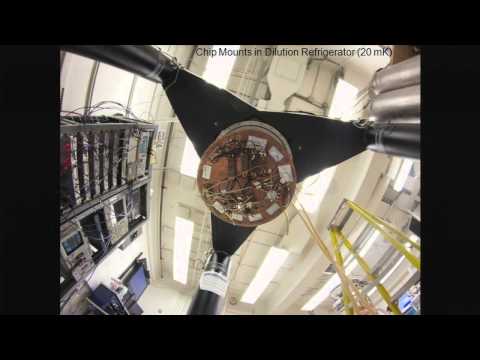
  • This is a picture, a graduate student lying on the ground

  • as he's putting it together in the dilution refrigerator.

  • These chips go inside this aluminum box.

  • And then coming out of it are coax wires

  • through some filters and other structures.

  • And then we have a lot of coax that

  • goes from here to the top of the cryostat at room temperature,

  • and then through the electronics over here.

  • And this is when it's open, you put a bunch of infrared shields

  • and a vacuum jacket around this and cool it down

  • with liquid helium.

  • And you can get to 20 millikelvin,

  • so that you get rid of all the electrical noise in the system.

  • And then it's just all controlled with all

  • these microwave electronics here, a lot of test equipment.

  • But everything is controlled over here by computer

  • so that it's easy to set up the experiment and get it to work.

  • So this is just some simple way to think about the qubits.

  • The first one we called a Rabi oscillation.

  • In this particular case, we take our coin

  • and we have it in the ground state.

  • And then, with microwaves, we flip the coin,

  • we rotate the coin at a steady rate that's

  • proportional to the microwave amplitude.

  • At a certain time, we stop the rotation

  • and then measure whether it's 0 or 1 state.

  • Of course, that's probablistic.

  • If it's going on edge, half the time it'll be heads

  • and half the time it'll be tails.

  • But you can do the experiment many times

  • to get a probability.

  • And what you see here is you just rotate longer and longer.

  • You're just flipping from heads to tails, 0 to 1, up and down.

  • And you see that the magnitude of the oscillation

  • doesn't decrease in time, because we

  • have very good coherence of the system.

  • So the typical time scale that we can flip the system

  • is maybe 10, 20 nanoseconds.

  • And then the tip of the lifetime of the system, which

  • is given here, where we go from 0 to 1,

  • and then we measure if it's in the 1 state versus time,

  • it eventually decays and relaxes to the 0 state.

  • But that does that in, say, 30 microseconds.

  • And the ratio between this and this is a factor of 1,000.

  • So we should be getting roughly a 0.1% error per gate.

  • And that would be, in principle, good enough

  • to do this error-corrected quantum computer.

  • But that's, of course, only in principle.

  • Actually, how do you make the gates?

  • So I want briefly to talk about the gates and what we do.

  • And I want to show you that we can make very complex gates.

  • And this system works extremely well.

  • And what we have here is something called

  • randomized benchmarking, where we're

  • putting in a very long sequence of gates into the system

  • and seeing if we're controlling the state.

  • Now, in this particular case, with randomized benchmarking,

  • we're going from 0 to 1 or from 0 to 0 plus 1, or 4 phases.

  • So this is going 6 equally spaced points

  • on this, what's called the block sphere.

  • So it's reduced-static quantum states.

  • But the nice thing about going to these particular set

  • of states and rotating or gating them into those states

  • is this forms a gate set that you can calculate very easily

  • just with classical computation.

  • And forms a generic base that you

  • can calculate very carefully and know what's going to happen.

  • So what we do here is we just take

  • a bunch of these different rotations

  • to take the state all around the block sphere,

  • over and over again.

  • And at the end, we know where it should be.

  • And then we rotate it back to pointing this way in the 0.

  • And we see if it's in the 0 state or not.

  • And then we do that complicated sequence of pulses

  • as shown here.

  • We then do it for other kind of gates

  • that move it in a different sequence.

  • And then average all that and say, OK,

  • do we get into the ground state?

  • And we see, of course, that it's not in the ground state

  • perfectly.

  • But then for you to have an error-- that's here,

  • and this is 0.1 size.

  • So this is not a huge error.

  • We can make hundreds and hundreds of gates

  • here in arbitrary combination, and we more or less

  • get this right answer here.

  • And you can work out the statistics.

  • And this says that the fidelity of these operations are 99.93%.

  • So only one gate in 1,000 is going

  • to give you a significant error.

  • And in fact, you can understand this a little bit more.

  • You can interleave these with specific gates

  • here, and very much quantify what's going on here.

  • But the end result here is we can make these quantum gates

  • well beyond the 99% that we need to do the surface

  • code and the error-free correction.

  • That's 1 qubit.

  • We have to run 2 qubits at the same time

  • to do some parallel processing.

  • We take those two qubits, set them at different frequencies.

  • Even though they're coupling here capacitively,

  • when you put it at 2 frequencies,

  • it effectively turns off the interaction.

  • You run your Clifford gates.

  • 99.9495 individually.

  • You then run them at the same time.

  • Because they're detuned, there's basically

  • no degradation in gate fidelity.

  • This number's smaller because you're

  • adding the errors of this and this in the way we do it.

  • So there's negligible crosstalk.

  • We should be able to operate these things in parallel.

  • We can also need to couple of them together.

  • We have to make this CNOT kind of gate

  • that I was talking about.

  • This, in fact, is the hard thing to do.

  • And this is what people have been trying to do for 20 years,

  • to get this gate good.

  • This is the hard gate.

  • And we think we've cracked this.

  • Conventional thinking-- you operate these qubits

  • in a very stable configuration so

  • that it's not frequency tunable.

  • It's like an atomic clock.

  • It gives the longest memory.

  • Then you connect them through some kind of quantum bus,

  • where that qubit connects to some resonator cavity,

  • connects to something else.

  • That gives you long-distance communication.

  • You then do some complex microwave or photon drive

  • to get all these things to interact and get it

  • to work [INAUDIBLE].

  • It's very complex And you get it to work.

  • Ion traps, for example, are at about 99%.

  • Superconducting qubits, when they do that,

  • these are slow gates.

  • 10 times slower than what I've been talking about.

  • Fidelity's not so great.

  • What we've done here is a totally different design.

  • We've taken all the conventional theory, the thinking,

  • and turned it on its head.

  • We use an adjustable frequency qubit.

  • And that's actually good, because we

  • can move them in and out of resonance

  • and turn on and off the interaction.

  • We have direct qubit coupling, no intermediate quantum

  • bus that can give us de-coherence.

  • And then, instead of driving it with microwaves or photons

  • we just change it with the DC pulse to change the frequency.

  • You need to do that accurately, but it can be done.

  • Theory says this should be really good, acceptable.

  • Experimentally, we do this.

  • These are some tuneup procedures.

  • It's for a Controlled-Z that's equivalent to the CNOT.

  • We can get this pi phase shift, this minus 1 side.

  • That's shown here.

  • This shows with full quantum states,

  • it's acting in a way it should be.

  • I'm running out of time, so I'm going to go over this quickly.

  • But basically, things are working right.

  • You do randomized benchmarking.

  • These are the Conrolled-Z gates.

  • We get a fast gate.

  • That's a very accurate 99.45, as shown here.

  • And sorry I can't go into this much.

  • This is best in the world.

  • It is better than ion traps.

  • Better than other qubits.

  • We know how to improve it.

  • This basic idea works very well.

  • Let me talk about qubit measurements.

  • I'll be done in four or five slides or so.

  • You have to measure the qubit.

  • What we have here is this qubit, and then it's capacitively

  • coupled to a microwave resonator right here.

  • And then that is also capacitively coupled

  • to another circuit right here.

  • So these being capacitively coupled,

  • it turns out that there's no energy

  • exchange between the qubit and here.

  • But the frequency of this particular resonator

  • changes depending on whether this is a 0 or a 1 state.

  • So what we do is we put a microwave signal here

  • that's resonant with this frequency that couples to that.

  • And because this frequency changes because of this

  • being the 0 and 1 state, that will

  • introduce a delay in this microwave

  • depending on whether it's a 0 or 1 state.

  • You then measure that with a quantum limited pre-amplifier

  • and room temperature analog-to-digital converter,

  • an FPGA that can measure the phase shift.

  • And you can tell what's going on in the system.

  • So here's just more details of that.

  • Here's the drive signal.

  • You put about 100 photons into that one resonator,

  • that has a frequency shift.

  • Here is plotted the real and imaginary part of the signal

  • that you're measuring here.

  • If you're in the 0 state, you have the phase,

  • so it's over here.

  • If you're in the 1 state, the phase is over here.

  • And integrating over about 100 nanoseconds,

  • you see these two signals are super well-separated.

  • And then you just say, if it's on this side,

  • it's a 0, and this side's a 1.

  • These are plots that are basically

  • showing what the separation error is.

  • Because these have Gaussian tails,

  • there are small errors between this.

  • But it basically says, in a few times

  • the operation of our single- or two-qubit operations,

  • we can see separation errors that are 10 to minus 2 to 10

  • to minus 3.

  • So we can measure the states extremely accurately.

  • Finally, we need to measure more than one qubit.

  • We talked about this one here.

  • We also have another qubit here with another resonator.

  • These are at two different frequencies.

  • So you put in two tones here.

  • This tone here gets shifted depending on the state.

  • This tone here gets shifted depending on this state.

  • You amplify that all.

  • The FPGA can separate out these two frequencies.

  • Get the amplitude and phase.

  • And then tell whether it's a 0 or 1 state.

  • So this is just data coming from-- this

  • is the readout signal of one qubit versus the other.

  • If we put a 0, 0 in here, this ends up here.

  • If it's 0, 1, it ends up here.

  • 1, 0 here.

  • 0, 1 here with the other states.

  • These states are all separated very nicely from each other.

  • So you can accurately measure multiple qubits

  • in a very short amount of time.

  • So we know how to scale that up.

  • And again, this is above the threshold.

  • Everything works well.

  • Last thing.

  • This is maybe people here will understand.

  • When you're building these complex systems,

  • you have to abstract away the functions.

  • You have a lot of complicated things going on here.

  • In our system, we can scale with all this stuff

  • with good control using software distraction, which

  • includes calibration of the hardware and waveform

  • and non-idealities.

  • Specific qubit calibrations.

  • So you basically calibrate the whole system.

  • And that takes, maybe, program 100,000 lines of code.

  • You understand that.

  • And then once you do all that, if you

  • want to do some complicated algorithm here, it's, what?

  • 7 lines of code.

  • You just say, I want to do these particular gates.

  • And all the calibrations are done for you.

  • You just put in the gates, run it, you're done.

  • So at this point, running the programs

  • are really essentially trivial, as it's all just calibrating it

  • up.

  • The amazing thing is that we can calibrate this up

  • and we run it, and it runs super well.

  • It runs with the errors that I showed you.

  • So it is possible to build this hardware system to abstract it

  • away as you would need to do.

  • So I think my 50 minutes is up.

  • I want to summarize and talk about the outlook.

  • People have been wanting to build a quantum

  • computer, a fault-tolerant quantum computer that

  • would potentially, eventually give you

  • enough exponential power.

  • We've been looking at this for 20

  • years in the experimental realm.

  • We think that our particular technology is now good enough

  • to do fault-tolerant computation.

  • This would be very hard to scale up.

  • We have a lot of technical challenges.

  • But the basic ingredients to do this are there.

  • It's at least good enough that we really

  • have to start doing this seriously.

  • No more playing around, writing physics papers-- although

  • were going to do that, too.

  • It's time to get serious and build this quantum computer.

  • The surface codes needs 99% fidelity.

  • We have 99.3, 99.5.

  • Measurement's good enough.

  • We think this is scalable.

  • Improvements are likely here so we can do well.

  • So the numbers are there.

  • It's time to get started.

  • What I'm looking at, based on what I've talked to here,

  • I would like to start what I think

  • is roughly a five-year project.

  • Although we can have problems.

  • It may take a little bit longer.

  • But I think we understand the basic technology.

  • And is basically to scale up to 100s,

  • maybe 1,000s of qubits using the surface code architecture.

  • And then try to do one with a logical error rate 10

  • to minus 15.

  • Hold the qubit state.

  • These incredible fragile quantum states and hold it

  • for 100 years or 1,000 years.

  • A really long time.

  • Showing that it would be OK.

  • And then this would be big enough so

  • that you can start doing these [INAUDIBLE] operation

  • or whatever to do logic operations at 10

  • to minus 6 errors.

  • I think this particular science project

  • is what's needed right now to show that all these ideas are

  • correct in a way that we understand

  • that the power is there.

  • And then, if this works, you would then go ahead

  • and, if you've got all the technology right,

  • you would try to build something that

  • was useful and could do something.

  • But we really want to focus on getting the science right

  • and understanding it in the next five years

  • and we really think that's doable.

  • Not just me.

  • All the graduate students and post-docs in my lab.

  • They're doing the work.

  • They really think this is possible along with me.

  • We look at the technology.

  • It really looks doable.

  • It looks like something we should be working hard on.

  • So let me end right there.

  • Here's our group at UC Santa Barbara.

  • It really takes a lot of people working together to do that

  • and we have a larger collaboration

  • of about 50 people with theorists

  • another experimentalists to get this done.

  • It's quite a lot of work, really takes a lot of teamwork.

  • But we think the technology's there.

  • So thank you very much.

  • [APPLAUSE]

  • MALE SPEAKER: Thank you, John.

  • It was a very nice talk.

  • I appreciate that you did it nicely in time,

  • so that leaves time for some questions.

  • JOHN MARTINIS: Yes.

  • AUDIENCE: Hi.

  • I was wondering if you could--

  • MALE SPEAKER: Could everybody use a microphone

  • so that people on the remote sites can hear it as well?

  • AUDIENCE: Hi.

  • I was wondering if you could compare your surface code

  • architecture with, for example, the toric code?

  • What are the advantages and disadvantages?

  • JOHN MARTINIS: Yeah.

  • The surface code architecture has the highest threshold

  • that we know of.

  • And that's incredibly important, because it's

  • hard to make good qubits.

  • We've been struggling with that.

  • Typically, initially, people talked about codes

  • with you needed 99.99% fidelities

  • to get it to threshold.

  • That, to me, looks really hard.

  • But at two 9s, that's something we can do.

  • The other nice thing about the surface code

  • is it only requires nearest neighbor interactions.

  • And if you're building that on the integrated circuit,

  • that's great.

  • So I think those two things are really

  • the key advantages of a surface code.

  • But people are looking at different codes

  • and different things.

  • And if something gets better, we can do that.

  • But surface code looks really quite ideal

  • for building integrated circuits.

  • AUDIENCE: Thank you.

  • JOHN MARTINIS: There's a question there.

  • MALE SPEAKER: Pass the microphone over there.

  • AUDIENCE: Can you discuss how far along you

  • are towards a surface code architecture,

  • and what is it going to take to get from 2 to 41?

  • Thanks.

  • JOHN MARTINIS: Yeah.

  • How far along?

  • So let's just look at the surface code.

  • Come on.

  • Slow computer.

  • You have to make a big array, OK?

  • Here, this is a couple hundred qubits.

  • There are some simple versions of the simple surface

  • code we can do at 5 or 9 qubits to test

  • if it's working properly.

  • And we're starting to design the chip.

  • And we hope to have some error detection, whatever,

  • working in about three to six months.

  • No one else is even thinking about doing that.

  • We think we can make quite rapid progress.

  • We really want to show that this simple surface

  • code is working right.

  • And then, at that point, I think people

  • will get on board that this is possible.

  • Everything is working great, so we really

  • think in three to six months we may have that.

  • And then we have to figure out how to make lots of qubits.

  • But we have some ideas.

  • We really want to demonstrate a simple version of that code.

  • MALE SPEAKER: I'm kind of scared to step

  • in front of the loudspeaker.

  • But connecting to this, I actually had one question.

  • You mentioned scaling it up would be really hard.

  • Can you list, a little bit, the main challenges?

  • JOHN MARTINIS: We know how to build, more or less,

  • the integrated circuit, and we know the materials.

  • But when you build something like this,

  • you have to get control lines in to all of those qubits.

  • Now, if you're talking about atoms

  • that are microns apart or less, it's

  • hard to get those control lines in.

  • But here, they're separated by hundreds of microns.

  • And we can IC fabricate control lines to get into that.

  • So we think we know how to do that.

  • We have an idea on how to do the processing and all that.

  • And then we have to bring 100 or 1,000 control lines

  • to the outside of a wafer, then wire-bond that up

  • to electronics at room temperature.

  • You just have to think like a high-energy physicist.

  • You just build a lot of wires and do all that.

  • We think we can do that.

  • From technology we have, or maybe

  • we just have to modestly invent something.

  • But that's the basic idea.

  • Just bring out those control wires

  • to the outside of the chip.

  • Wire-bond them.

  • All these cables going up to racks of electronics.

  • And for doing the scientific demonstration,

  • we think we can do that.

  • Eventually, if you want to go beyond the thousand qubits,

  • you have to put the control either right down in the chip.

  • And that there is the technology of classical Josephson junction

  • computing, which people have been working on

  • for years and years.

  • And we actually have a program to start

  • trying to figure out how to do that.

  • So as we're building up this brute-force way,

  • at the same time, we wanted to be developing

  • the classical control circuitry to do that.

  • Going back to D-Wave, one of the impressive things

  • D-Wave has done is they built that classical control.

  • It's not exactly what we want.

  • But when I look at what they invented,

  • it gives me a lot of hope that we can figure that out.

  • Because that's both a combination

  • of analog and digital.

  • We have to do the research.

  • But I'm optimistic that that can all be done.

  • It's just hard.

  • But OK.

  • This is what you have to do.

  • And in fact, the hard part of building a quantum computer--

  • making good qubits, DiVincenzo criteria-- yeah,

  • it's really hard to get 99.45% fidelity.

  • The hard part is the control circuitry.

  • You have millions of qubits.

  • How do you get all that control within each qubit?

  • Because it's basically analog control.

  • I think you can do it here.

  • But that's going to be a super challenge.

  • Again, to do some physics, we don't have to crack that yet.

  • MALE SPEAKER: Another immediate thought.

  • That if you could borrow some of the control electronics from

  • D-Wave and apply it here--

  • JOHN MARTINIS: Their control electronics

  • is a different mode than this.

  • But there could be a lot of commonality.

  • And for me, it's more that they've

  • shown that you can mix digital and analog, in their way.

  • And you might want to borrow some of the ideas

  • or be inspired by those ideas to do it.

  • But I really feel that, given people working hard on that,

  • we can crack that problem.

  • But it's something eventually we do.

  • However, if we want to show the science works well,

  • and to have a fragile qubit state

  • and hold it for 100 years, I think you can brute force that.

  • Which is one path we want to take.

  • And then, at the same time, work on the other things.

  • That's my view of how things should go.

  • MALE SPEAKER: There was one more question earlier,

  • but I think we--

  • AUDIENCE: I have a question.

  • JOHN MARTINIS: Yes.

  • AUDIENCE: So how small can you make this, practically,

  • if you wanted to have-- and you show a homogeneous matrix here.

  • But if you wanted to have a bunch of matrices,

  • maybe with some space between them for control circuitry.

  • This is 10 by 10, the minimum size.

  • JOHN MARTINIS: So that's what I'm talking about here.

  • Right now, we're thinking the cell size

  • is going to be eventually between 100

  • microns to a millimeter on a size.

  • And remember, it can't be too small,

  • because you have to pack all that control circuitry in it.

  • So at 100 microns in a millimeter,

  • you can put a significant amount of control circuitry.

  • And then, if you do that, say 100 microns,

  • it's maybe meters across in this direction.

  • It'd have to be a big thing.

  • But those are the numbers.

  • Everyone thinks, from modern microelectronics,

  • that you have to make everything small.

  • But as soon as you do that, you have

  • to make your control circuitry that small.

  • And the control circuitry is not two transistors or something.

  • It's complicated.

  • So that's why you need it kind of big.

  • But these numbers, I think, you can imagine, given enough time,

  • you can solve these problems.

  • They're not easy problems.

  • But I think it's possible.

  • Yeah.

  • AUDIENCE: About, basically, the oral architecture

  • of the computer.

  • So suppose you placed 100 qubits on the chip and all the control

  • circuitry.

  • Does that mean that you already have a 100-qubit computer?

  • So is this a device for practical computations?

  • Or, basically, the difference between physical and logical

  • qubits here.

  • What is that?

  • JOHN MARTINIS: It depends if you're

  • worried about error correction in your algorithm.

  • And that's a question we're talking

  • about today, as we did here.

  • I'm talking about building an error-corrected device.

  • So if you build 1,000 qubits, your error rate

  • is going to be 100 years.

  • But then you could start making smaller qubits in it,

  • where their error rate may be one per second.

  • But then you could do logical operations

  • with those qubits and test things.

  • So I'm not sure if you could do anything practical

  • at that point.

  • But you can certainly test the science.

  • And that's what I'm thinking right now.

  • Like with the D-Wave, the question is the science of it.

  • So if we were to test out the science

  • and make sure that everything was OK,

  • that would give us a lot of confidence

  • that we can move forward in doing it.

  • Because there's a lot of theoretical assumptions

  • here that we have to deal with.

  • But you might be able to use such an array

  • without error-corrected mode in some interesting, useful way.

  • And then we would, of course, do that,

  • if someone had a good plan.

  • But the error correction forces you into an architecture.

  • But once we have the technology, we

  • can do other things, for sure.

  • For example, part of our group is

  • looking at quantum simulation for a physics problem.

  • And we're thinking we can do some interesting things there

  • now.

  • MALE SPEAKER: Maybe just to quickly check

  • whether any of the remote sites may have a question?

  • There don't seem to be.

  • JOHN MARTINIS: OK.

  • AUDIENCE: Sorry, ask the question again?

  • MALE SPEAKER: I was wondering if the remote sites, was there

  • any questions from there?

  • OK.

  • Any last question from here?

  • Thanks one more time--

  • JOHN MARTINIS: Thank you very much.

  • MALE SPEAKER: --for the very interesting talk.

  • And very upbeat information.

  • JOHN MARTINIS: Good.

  • Thank you.

  • [APPLAUSE]

MALE SPEAKER: Good afternoon.

Subtitles and vocabulary

Click the word to look it up Click the word to find further inforamtion about it